01. Collision Detection Basics
Collision Detection Basics
ND313 C03 L02 A01 C21 Intro
The Collision Detection Problem
A collision avoidance system (CAS) is an active safety feature that warns drivers or even triggers the brake in the event of an imminent collision with an object in the path of driving. If a preceding vehicle is present, the CAS continuously estimates the time-to-collision (TTC). When the TTC falls below a lower threshold, the CAS can then decide to either warn the driver of the imminent danger or - depending on the system - apply the vehicle brakes autonomously. For the engineering task you will be completing in this course this means that you will need to find a way to compute the TTC to the vehicle in front.
Let us take a look at the following scene:
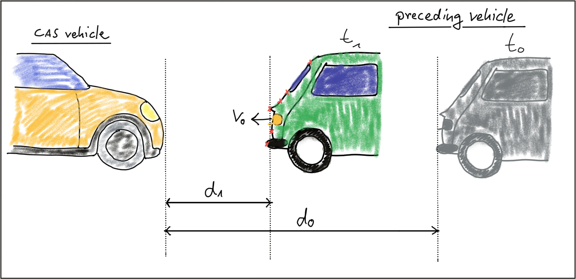
In this traffic scenario, the green vehicle starts to reduce its speed at time t_0 , which is when the yellow vehicle, equipped with a collision sensor, takes the distance measurement d_0 . A moment later, at time t_1 , the green vehicle is considerably closer and a second measurement d_1 is taken. The goal now is to compute the remaining TTC so the system can warn the driver of the yellow vehicle or even trigger the brakes autonomously.
Before we can do this however, we need to find a way to describe the relative motion of the vehicles with a mathematical model.
Constant velocity vs. constant acceleration
To compute the TTC, we need to make assumptions on the physical behavior of the preceding vehicle. One assumption could be that the relative velocity between the yellow and green vehicle in the above figure were constant. This would lead to the so-called constant velocity model (CVM) which is represented by eq. 1 in the following diagram.
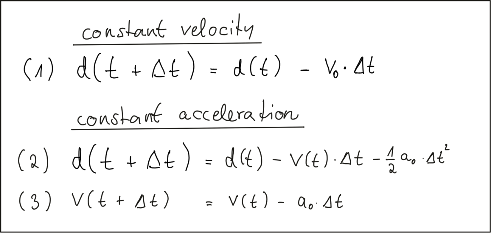
As you can see, the distance to the vehicle at time instant t + \Delta t is smaller than at time t , because we subtract the product of a constant relative velocity v_0 and time \Delta t . From an engineering perspective, we would need a sensor capable of measuring the distance to the preceeding vehicle on a precisely times basis with a constant dt between measurements. This could very well be achieved with e.g. a Lidar sensor.
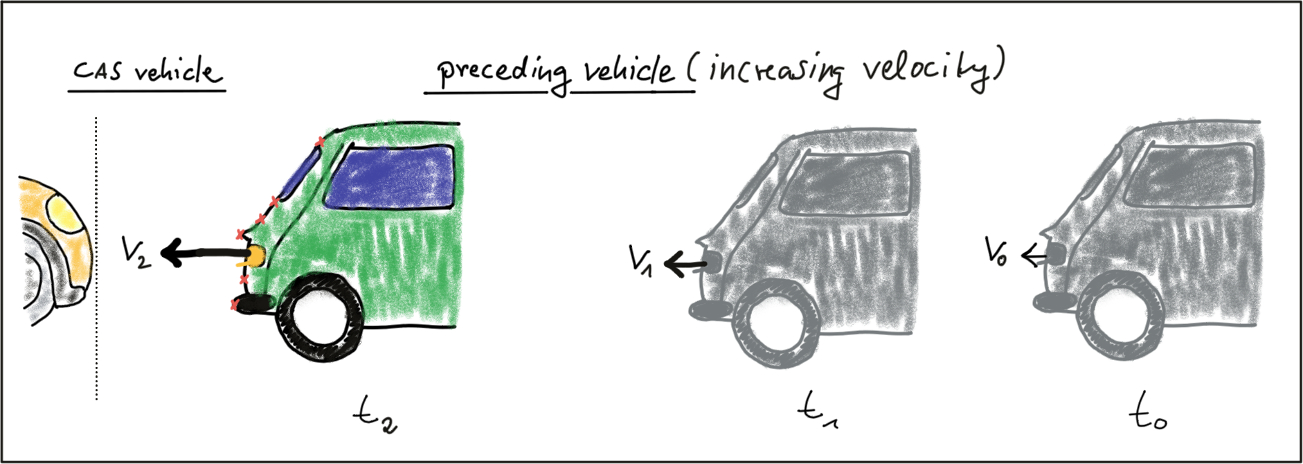
Especially in dynamic traffic situations where a vehicle is braking hard, the CVM is not accurate enough however, as the relative velocity between both vehicles changes between measurements. In the following figure, the approaching vehicle is shown at three time instants with increasing velocity.
We can thus expand on our CVM by assuming velocity to be a function of time and subtract a second term in eq. 2 which is the product of a constant acceleration and the squared time dt between both measurements. Eq. 3 displays velocity as a function of time, which is also dependent on the constant acceleration we used in eq. 2. This model is referred to as constant acceleration model (CAM) and it is commonly used in commercially available collision detection systems. On a side note, if we were using a radar sensor instead of a Lidar, a direct measurement on velocity could be taken by exploiting a frequency shift in the returning electromagnetic wave due to the Doppler effect. This is a significant advantage over sensors such as Lidar, where velocity can only be computed based on (noisy) distance measurements.
In this course, we will be using a CVM instead of the CAM as it is much simpler to handle with regard to the math involved and with regard to the complexity of the programming task ahead of you. For small instances of dt we will assume that the CVM model is accurate enough and that it will give us a decent estimate of the TTC. Should you be involved in building a commercial version of such a system at a later stage in your career however, keep in mind that you should be using a constant acceleration model instead.
ND313 C03 L02 A01b C21-A4